Lec 05: Data Structures

1. Resizing arrays

1.1. How to resizing arrays

We already know that array is a contiguous spaces in computer's memory in which we could store values, and we use malloc to acquire a chunk of memory from system for the array.

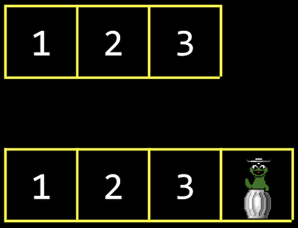
But once we get memory through malloc, the size of arrays is fixed. If there is some input but our array haven't enough memory for those extra inputs, we have to resize our array.

One solution is to allocate more memory where there's enough space, and then move our original array there. But it will need more time to copy our array to new space, which becomes an operation with running time of O(n).

And the lower bound of inserting an element into an array would be O(1), since we might already have enough space in the array for storing it.

1.2. Implementing resizing arrays

Let's see how we might implement resizing an array:

#include <stdio.h>
#include <stdlib.h>
const int N = some_integer;

int main (void)
{
    // suppose we already have an array with N integer values
    int *list = malloc(N * sizeof(int));
    // Now we want to store another value, that is to resize this array

    // Fisrt allocate more memory to store extra value
    int *tmp = malloc((N + 1) * sizeof(int));
    if (tmp == NULL) {
        // free the memory that we allocated before exit the program
        free(list);
        return 1;
    }
    // copy original list to tmp
    for (int i = 0; i < N; i++) {
        tmp[i] = list[i];
    }
    // Now we can store new integer
    tmp[N] = new_number;
    // Free the original list which won't be used anymore
    free(list);
    // Point to new list
    list = tmp;
    // Free all the memory we allocated before we exit the program
    free(list);
    return 0;
}

We can see it's troublesome if we handling this process ourselves. Therefore, C provides a function realloc, to reallocate some memory that we allocate earlier from heap areas using malloc.

int *tmp = realloc(list, (N + 1) * sizeof(int));

And realloc copies our old array, list, for us into a bigger chunk of memory of the size we pass in.

If there happens to be spaces after out existing chunk of memory, we'll get the same address back, but with the memory after it allocated to our variable as well.

2. Data structures

Data structures are more complex ways to organize data in memory, allowing us to store information in different layouts.

To build a data structure, we'll need some tools:

• struct to create custom data types
• . to access properties in a structure
• * to go to an address in memory pointed by a pointer
• -> to access properties in a struct pointed by a pointer

3. Linked list

3.1. What is linked list

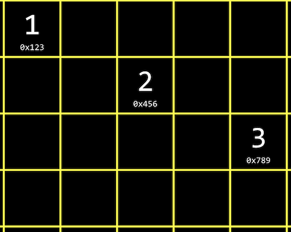
With a linked list, we can store a list of values that can easily be grown by storing values in different parts of memory.

E.g. we have the values 1, 2 and 3, each at some address in memory like 0x123, 0x234, and 0x345, which are not contiguous addresses. So it's different than the array, that is we can use whatever locations in memory that are free.

3.2. How to implement

Due to these address are not contiguous in memory, we cannot track them by indexing addresses. So we need link our list together by allocating, for each element, enough memory for both the value we want to store, and the address of the next address.

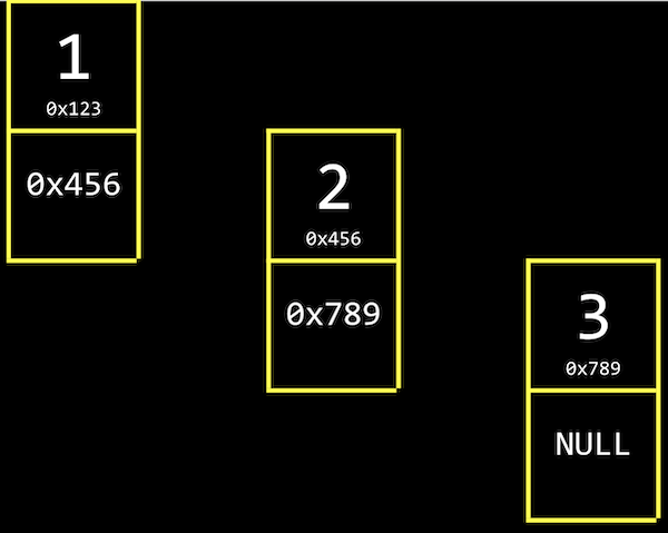
We'll call it a node, which a component of our data structure that stores both a value and a pointer. As we mentioned before, we'll implement out nodes with a structure.

And notice that, the last node of linked list, we have the null pointer since there's no next element. When we need to insert another node, we just change the single null ptr to point our new node.

3.3. Trade off

We have the trade off of needing to allocate twice as much memory for each element, in order to spend less time adding values.

And we no longer can use binary search, which depends on the index of address yet our nodes might be anywhere in memory.

3.4. Implementing nodes

Before we implement linked lists, we have to implement the component of linked lists, nodes.

In code, we might want to create our own struct called node, and we need to store both our value, an int called number, and a pointer to the next node, called next.

typedef struct node {
    int number;
    struct node* next;
}
node;

Notice that we start with typedef struct node so that we can refer to a node inside our struct.

3.5. Implementing linked lists

#include <stdio.h>
#include <stdlib.h>

// Represent a node
typedef struct node {
    int number;
    struct node *next;
}
node;

int main (void)
{
    // List of size 0. We initialize the value to NULL explicitly, so there's no
    // garbage value for our list variable
    node *list = NULL:

    // Allocate memory for a node, n
    node *n = malloc(sizeof(node));
    if (n == NULL) {
        return 1;
    }

    // Set the value and pointer to our node
    n->value = N;
    n->next = NULL:

    // Add node n by pointing list to it, since we only have one node so far
    list = n;

    // Allocate memory for another node, and we can reuse our variable n to point
    // to it, since list points to the first node alraedy
    n = malloc(sizeof(node));
    if (n == NULL) {
        free(list);
        return 1;
    }
    // Set the values in our new node
    n->number = N;
    n->next = NULL;

    // Update the pointer in our first node to point to the second node
    list->next = n;

    // Allocate memory for the third node
    n = malloc(sizeof(node));
    if (n == NULL) {
        // free both of our other nodes
        free(list->next);
        free(list);
        return 1;
    }

    // Follow the next pointer of the list to the second node, and update
    // the next pointer there to point to n
    list->next->next = n;

    // Print list using a loop, by using a temporary variable, tmp, to point
    // to list, the first node. Then, every time we go over the loop, we use
    // tmp = tmp->next to update our temporary pointer to the next node.
    // We might keep going as tmp points somewhere, stopping when we get the last 
    // node and tmp->next == null, namely there's no more nodes after this node.
    for (node *tmp = list; tmp != NULL; tmp = tmp->next) {
        printf("%i\n", tmp->number);
    }
    // Free list, by using a while loop and a temporary variable to point to
    // the next node before freeing the current one.
    while (list != NULL) {
        // Point to the next node first
        node *tmp = list->next;
        // Then, free the first node
        free(list);
        // Now we can set the list point to the next node
        list = tmp;
    }
}

If we want to insert a node to the front of our linked list, we should need to carefully update our node to point to the one following it, before updating the list variable. Otherwise, we'll lose the rest of our list.

// Here, we're inserting a node into the front of the list, so we want its next
// pointer to point to the orginal list. Then we can change the list to point to n.
n->next = list;
list = n;

That is, at first we'll have a node with value 1 pointing to the start of our list, a node with value 2.

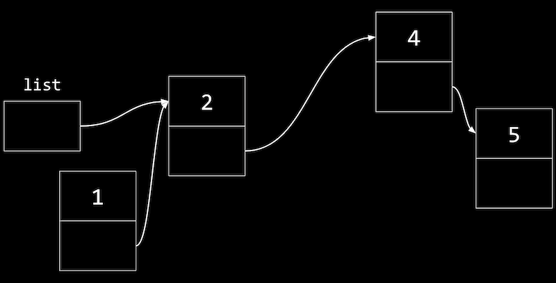
Now we can change our list variable to point to the node with value 1, and not lost the rest of our list.

Similarly, to insert a node into the middle of our list, we can change the next pointer of new node first to point to the rest of the list, then update the previous node to the new node.

A linked list demonstrates how we can build flexible data structure in memory, though we're only visualizing it in one dimension.

4. Tree

4.1. What is Tree

With a sorted array, we can use binary search to find an element, starting at the middle (the yellow one), then the middle of either half (red), and finally left or right (green) as needed.

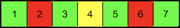
With an array, we can randomly access elements in O(1) time, since we can use arithmetic to go to an element at any index.

A tree is another data structure where each node points two other nodes, one to the left (with a smaller value) and one to the right (with a larger value).

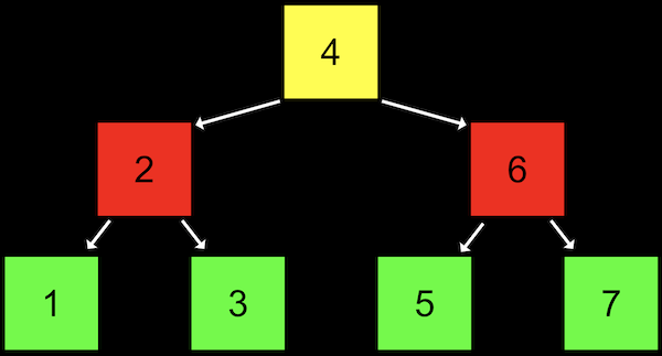
Notice that we now visualize this data structure in two dimensions (even though the nodes in memory can be at any location).

And we can implement this with a more complex version of a node in a linked list, where each node has not one but two pointers to other nodes. All the value to the left of a node are smaller, and all the value to the right are greater, which allows this to be used as a binary search tree. And the data structure is itself defined recursively, so we can use recursive functions to work with it.

Each node has at most two children, i.e. nodes it's pointing to.

4.2. Implementing Binary Search Tree

Like a linked list, we'll want to keep a pointer to just the beginning of the list, but in this case we want to point to the root, or top center node of the tree (4 in this case).

We can define a node with not one but two pointers:

typedef struct node {
    int number;
    struct node *left;
    struct node *right;
}
node;

And write a function to recursively search a tree:

// tree is pointer to a node that is the root of the tree we're searching in.
// number is a value we're trying to find in the tree.
bool search (node *tree, int value) {
    // Fisrt, make sure that the tree isn't NULL, if we're reached a node on the
    // bottom, or if our tree is entirely empty.
    if (tree == NULL) {
        return false;
    }
    // If we're looking for a number that's less than the tree's number, search the
    // left side, using the node on the left as the new tree.
    else if (number < tree->number) {
        return search(number, tree->left);
    }
    // Otherwise, search the right side, using the node on the right as the new tree.
    else if (number > tree->number) {
        return search(number, tree->right);
    }
    // Finally, we've found the number we've looking for, so we can return true.
    // We can simplify this to just "else", since there's no other case possible
    else if (number == tree->number) {
        return true;
    }
}

4.3. Trade off

With a binary search tree, we've incurred the cost of even more memory, since each node now needs space for a value and two pointers. Inserting a new value would take O(log n) time, since we need to find the nodes that it should go between.

If we add enough nodes, though, our search tree might start to look like a linked list:

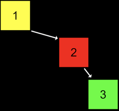
That is, we started our tree with a node with value 1, then added the node with value 2, and finally added the node with value 3. Even though this tree follows the constraints of a binary search tree, it's not as efficient as it could be.

We can make this tree balanced, or optimal, by making the node with value 2 the new root node. More advanced courses will cover data structures and algorithms that help us keep trees balanced as nodes are added.

5. More data structures

5.1. Hash table

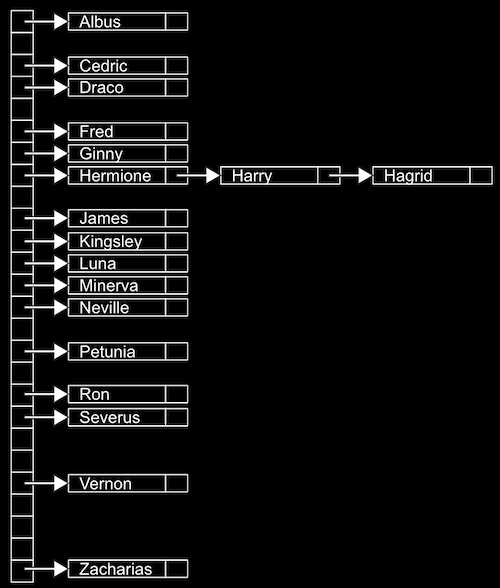
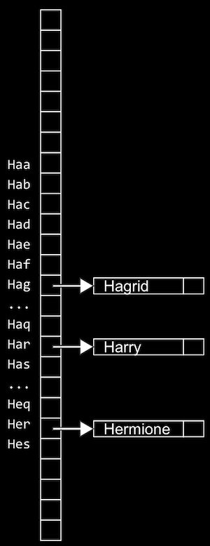
A data structure with almost a constant time, O(1) search is a Hash table, which is essentially an array of linked lists. Each linked list in the array has elements of a certain category.

E.g., we might have lots of names, and we might sort then into an array with 26 positions, one for each letter of the alphabet.

Since we have random access with arrays, we can set elements and index into a location, or bucket, in the array quickly.

A location might have multiple matching values, but we can add a value to another value since they're nodes in a linked list, as we see with Hermione, Harry, and Hagird. We don't need to grow the size of our array or move any of our other values.

This is called hash table because we use a hash function, which takes some input and deterministically maps it to the location it should go in. In our example, the hash function just returns an index corresponding to the first letter of the name, such as 0 for "Albus" and 25 for "Zacharias".

But in the worst case, all the names might start with the same letter, so we might end up with the equivalent of a single linked list again. We might look at the first two letters, and allocate enough buckets for 26*26 possible hashed values, or even the first three letters, requiring 26*26*26 buckets.

Now, we're using more space in memory, since more of those buckets will be empty, but we're more likely to only need one step to look for a value, reducing our running time for search.

To sort some standard playing cards, too, we might first start with putting them in piles by suit, of spades, diamonds, hearts, and clubs. Then, we can sort each pile a little more quickly.

It turns out that the worst case running time for a hash table is O(n), since, as n gets very large, each bucket will have on the order of n values, even if we have hundreds or thousands of buckets. In practice, though, our running time will be faster since we’re dividing our values into multiple buckets.

5.2. Trie

We can use another data structure called a trie, (pronounced like "try", and is short for "retrieval").

A trie is a tree with arrays as nodes.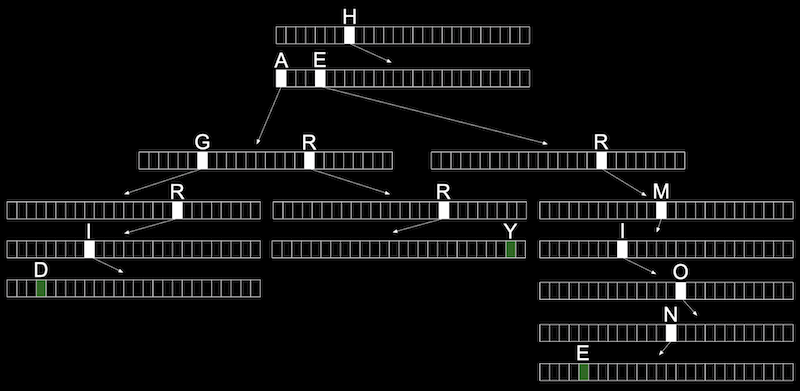

In this case, each array will have each letter, A-Z, stored. For each word, the first letter will point to an array, where the next valid letter will point to another array, and so on, until we reach a boolean value indicating the end of a valid word, marked in green above. If our word isn’t in the trie, then one of the arrays won’t have a pointer or terminating character for our word.

Now, let's consider the trade off for this data structure, even if our data structure has lots of words, the maximum lookup time will be just the length of the word we’re looking for. This might be a fixed maximum, so we can have O(1) for searching and insertion.

The cost for this, though, is that we need lots of memory to store pointers and boolean values as indicators of valid words, even though lots of them won’t be used.

5.3. Abstract data structures

There are even higher-level constructs, abstract data structures, where we use our building blocks of arrays, linked list, hash tables, and tries to implement a solution to some problem.

5.4. queue

For example, one abstract data structure is a queue, like a line of people waiting, where the first value we put in are the first values that are removed, or first-in-first-out (FIFO). To add a value we enqueue it, and to remove a value we dequeue it.

This data structure is abstract because it’s an idea that we can implement in different ways: with an array that we resize as we add and remove items, or with a linked list where we append values to the end.

5.5. Stack

An “opposite” data structure would be a stack, where items most recently added are removed first: last-in-first-out (LIFO). At a clothing store, we might take, or pop, the top sweater from a stack, and new sweaters would be added, or pushed, to the top as well.

5.6. Dictionary

Another example of an abstract data structure is a dictionary, where we can map keys to values, such as words to their definitions. We can implement one with a hash table or an array, taking into account the tradeoff between time and space.

---

最后更新: April 23, 2022